
写在前面
在NUS的学习过程中所涉及到的一些Assignments,会陆陆续续整理然后放上来,由于是英语书写同时也为了锻炼自己的英文写作,遂会尽量用英文来写整个的过程(其实也是照抄作业而已)。本Assignment是关于IMDB5000电影评分的一个分析,比较偏入门的一个作业,通过这个作业可以对R中重要的可视化作图模块有一个较为整体的认识。
Introduction
IMDB 5000 is an Internet movie database with highest rated TV series with at least 5000 votes. In this task, IMDB 5000 is implemented as our database to explore and visualize the different distributions depending on various factors. This dataset could be found in data.world or Kaggle dataset, which includes 28 factors and 5043 movies. The metadata is listed below:
| Variables | Variables | Variables | Variables |
|---|---|---|---|
| color | actor_2_facebook_likes | actor_3_name | budget |
| director_name | movie_facebook_likes | facenumber_in_poster | title_year |
| num_critic_for_reviews | gross | imdb_score | aspect_ratio |
| duration | genres | plot_keywords | content_rating |
| director_facebook_likes | actor_1_name | movie_imdb_link | cast_total_facebook_likes |
| actor_3_facebook_likes | movie_title | num_user_for_reviews | actor_1_facebook_likes |
| actor_2_name | num_voted_users | language | country |
Objectives
The objective of this report is to answer the following questions based on the IMDB 5000 dataset:
- What is the trend for number of movies produced annually, and their
corresponding IMDB scores? - What are the popular movie genres based on IMDB scores?
- What are the national trends for movies and their corresponding quality?
- How does budget and mean gross impact IMDB scores?
- Who are the most prolific directors, while which directors have the highest reputation?
Data Clean
The dataset was first checked to ensure that there were no missing values. Movie title and IMDB score was treated as essential data in the dataset, and duplicated movies with the same title, excluding the series movies that may have the same title, were removed. After omitting 45 movies, 4998 movies remain.
- It was observed during data cleaning that all movies titles contained the unknown character “Â “. As such, “movie_title” column was formatted to remove this.
splitFun <- function(x) strsplit(x, '\302')[[1]][1]
cleaned_titles = sapply(titles, splitFun)
Visualization
This part was aimed to answer the questions declared in objectives.
Question 1: Annual movies general quantity and quality
What is the trend for number of movies produced annually, and their corresponding IMDB scores?
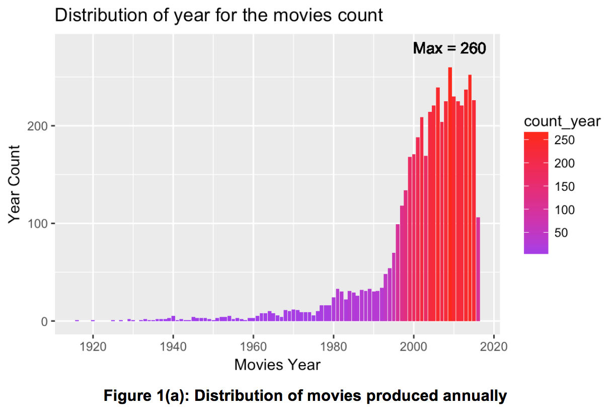
The subset of dataset was selected from year of 1980. The movies count versus years was compiled in R. Using geom_text to add the maximum point in the plot.
q1_data_greater_1980 = q1_data[as.numeric(q1_data$title_year) > 1980, ]
q1_data %>%
  group_by(title_year) %>%
  summarise(count_year = n()) %>%
  ggplot(aes(x = title_year, y = count_year, fill = count_year)) +
  geom_bar(stat = "identity") +
  geom_text(aes(2009, 280, label = "Max = 260" )) +
  labs(x="Movies Year", y="Year Count") +
  ggtitle("Distribution of year for the movies count") +
  scale_fill_gradient(low = "purple", high = "red")
Furthermore, the median score of annual movies versus different years was plot using ggplot. geom_smooth() was used to smooth the tendency line to describe the general relationship.
q1_data %>%
  group_by(title_year) %>%
  summarise(mean_score = mean(imdb_score)) %>%
  ggplot(aes(x = title_year, y = mean_score, group = 1)) +
  geom_point() +
  geom_line() +
  geom_smooth() +
  labs(x="Movies Year", y="Mean IMDB score every year") +
  ggtitle("Mean IMDB score for each year")
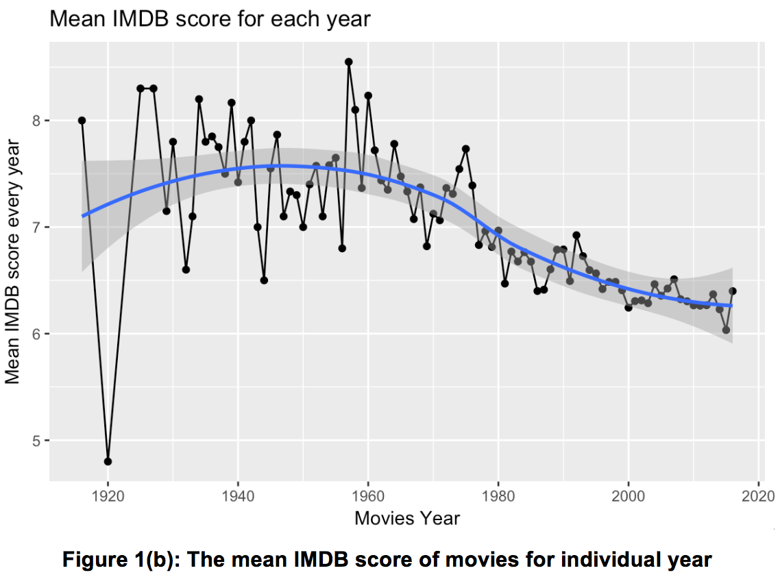
Figure 1(a) illustrates the distribution of movies produced annually. It’s noted that before 1980, the overall quantity of movies produced was relatively low. From 1980 to the mid-1990s, we note a gradual increase in the number of movies produced. Since the mid-1990s however, the movie market grew tremendously, reaching a high of 260 in 2009.
The figure 1(b) illustrates the annual mean IMDB scores points, with the best fit line indicated in blue. From the graph, it’s observed that the mean IMDB score has been increasing before 1950. After 1950 however, the mean IMDB scores has been reducing over the years, reaching an all-time low of 6 in 2015, the lowest since 1960.
From the above trends, it’s evident that even though the movie industry has been growing exponentially over the years, these do not correspond with an increase in the mean IMDB scores. This means that there has been a significant number of low quality movies. Consequently, it’s also observed that people enjoy classical movies from the early years.
Question 2: Popular movie genres.
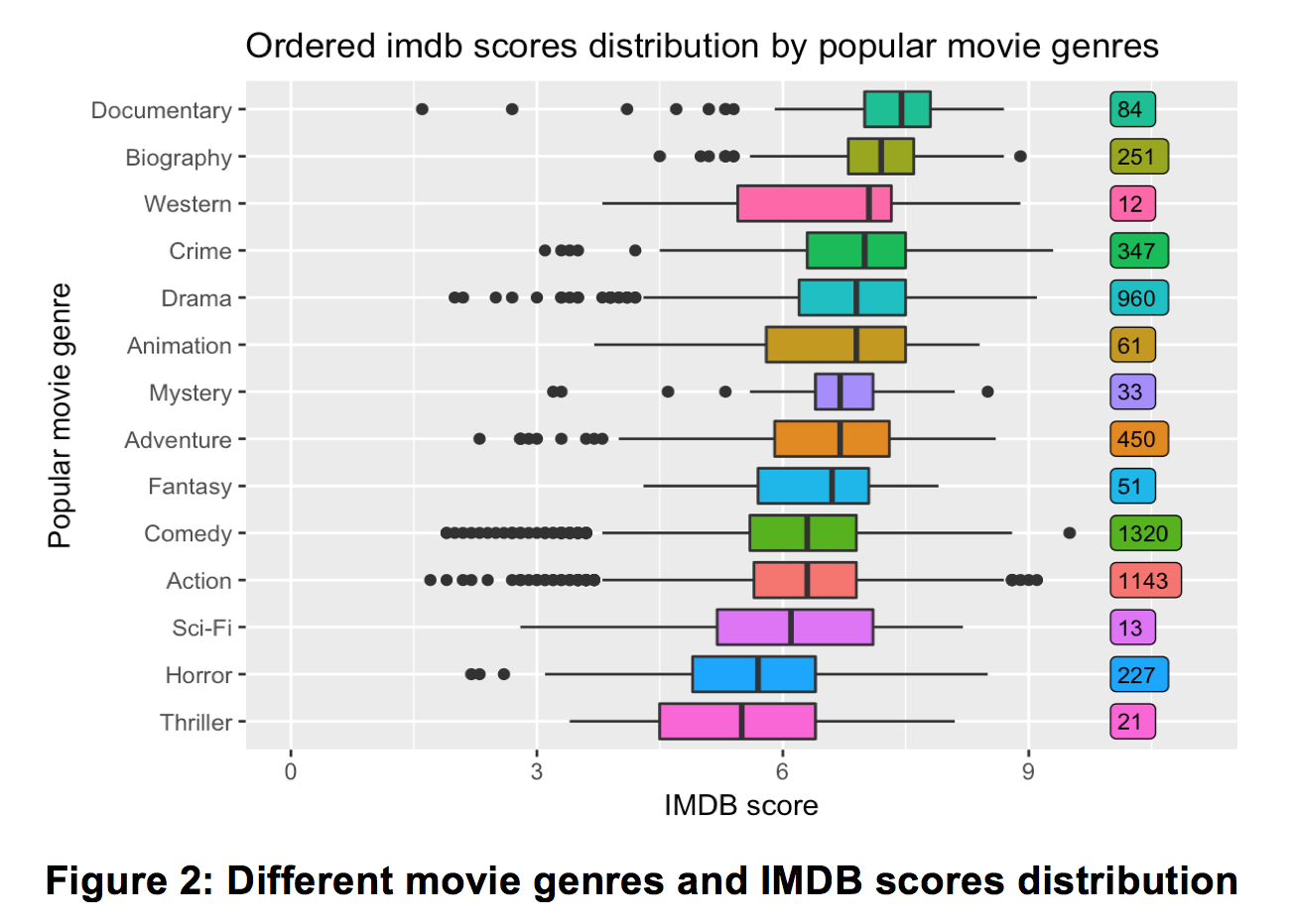
To answer this question, some additional data cleaning beyond those stated in section 3.1 was done, as there were some genres that were separated by a vertical line (“|”). These genres were split, and the first genre was considered as the primary genre. This left us with 21 genres.
judgeAndSplit <- function(x) {
  sp = strsplit(x, '[|]')[[1]][1]
  return(sp)
}
genres_name = as.character(movies$genres)
movies = movies %>%
  mutate(genres1 = as.factor(sapply(genres_name, judgeAndSplit)))
Since we’re interested in popular genres, genres with more than 10 movies were selected, resulting in 14 key genres selected. With these genres, a boxplot was generated in Figure 2. Note that these genres were arranged in descending order in terms of their median IMDB scores.
typeLabelCount = q2_modified %>%
  group_by(genres1) %>%
  summarise(count = n()) %>%
  as.data.frame()

q2_modified %>%
  ggplot(aes(reorder(genres1, imdb_score, median, order = TRUE), y = imdb_score, fill = genres1)) +
  geom_boxplot() +
  coord_flip() +
  geom_label(data = typeLabelCount, aes(x = genres1, y = 10, label = count),  hjust = 0, size = 3) +
  ggtitle("Ordered imdb scores distribution by popular movie genres") +
  guides(fill=FALSE) +
  ylim(0, 11) +
  labs(x = "Popular movie genre", y = "IMDB score")
From the figure 2 below, the most popular genre was “Documentary”, achieving a median score nearly 7 with 84 movies. The least popular genre out of the 14 key genres selected was “Thriller”, with a median score of around 5 out of of 21 movies. While the “Comedy” and “Action” genres had the largest numbers, the overall IMDB score performances were still poor.
As such, we conclude that genres such as “Documentary”, “Biography”, “Western”, “Crime” and “Drama”, which are adapted either from reality or original novels, tend to perform have higher scores.
Question 3: National movies quality
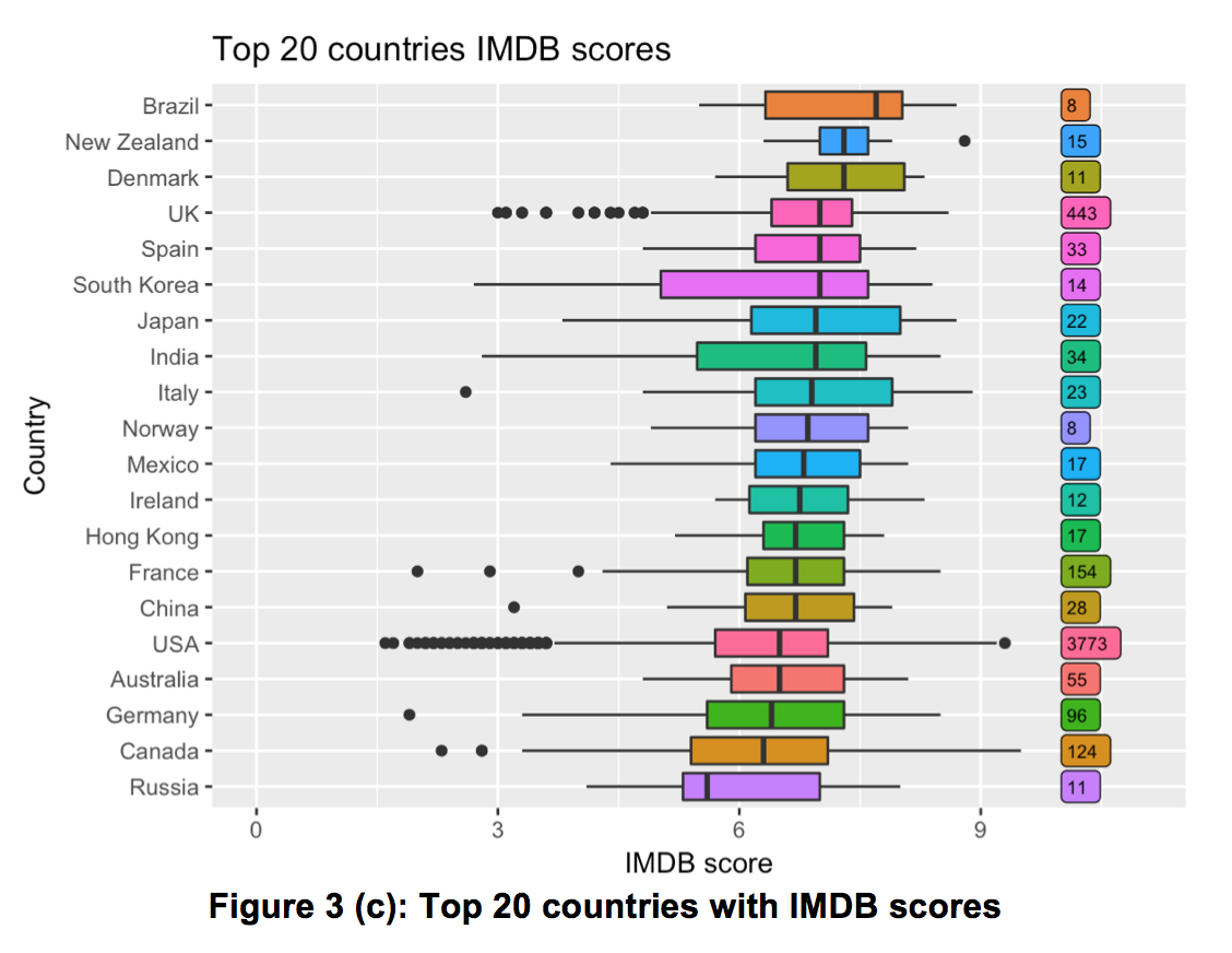
In this part, the top 20 countries that produced the most movies were considered, thus demostrated the IMDB scores condition.
q3_data[q3_data$country %in% countriesTopList$country, ] %>%
  ggplot(aes(reorder(country, imdb_score, median, order = TRUE), imdb_score, fill = country)) +
  geom_boxplot() +
  coord_flip() +
  guides(fill=FALSE) +
  geom_label(data = as.data.frame(q3_top20_cny), aes(x = country, y = 10, label = country_count), hjust = 0, size = 2.5) +
  labs(x = "Country", y = "IMDB score", title = "Top 20 countries IMDB scores") +
  ylim(0, 11)
From Figure 3, we observe that although USA had the highest movie quantity (3773) and took up more than 75% of the dataset, it only achieved a rank of 16th in the IMDB median scores ranking. If we considered the quality of the movies produced, the country with the highest median score is Brazil, and the lowest is Russia. If we consider both quantity and quality of movies produced, movies from the UK movies had a comprehensively good performance (2nd in quantity, 4th in median scores ranking) amongst all the countries.
Question 4: Budget and mean gross impact IMDB scores
To explore the effect of budget and mean gross to IMDB scores, a new factor named “IMDB score level” was defined, with 0.5 as the score step. This serves to round the IMDB scores to the nearest 0.5. Based on this, the movies’ mean budget and gross belonging to corresponding score levels were calculated. The results are as plotted in a line chart shown in Figure 4 (a) and (b).
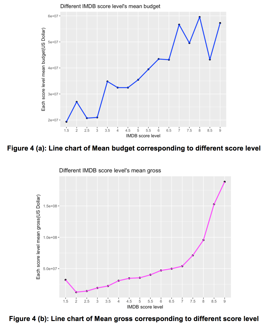
From figure 4 (a) and (b), we conclude that IMDB scores are positively correlated to budget and gross. Furthermore, movies with a higher score on IMDB tend to do better at the box office. If a movie is expected to have a high score, more financial support should be available in the early stage.
q4_data = movies
q4_cleaned_data = q4_data %>%
  subset(!is.na(gross)) %>%
  subset(!is.na(budget))

q4_cleaned_data %>%
  group_by(imdb_score_level) %>%
  summarise(score_count = n(),
            mean_budget = mean(budget, na.rm = TRUE)) %>%
  ggplot() +
  geom_point(aes(x = as.factor(imdb_score_level), y = mean_budget)) +
  geom_path(aes(x = as.factor(imdb_score_level), y = mean_budget, group = 1), size = 1, color = 4) +
  labs(x = "IMDB score level", y = "Each score level mean budget(US Dollar)", title = "Different IMDB score level's mean budget")

q4_cleaned_data %>%
  group_by(imdb_score_level) %>%
  summarise(score_count = n(),
            mean_gross = mean(gross, na.rm = TRUE)) %>%
  ggplot() +
  geom_point(aes(x = as.factor(imdb_score_level), y = mean_gross)) +
  geom_path(aes(x = as.factor(imdb_score_level), y = mean_gross, group = 1), size = 1, color = 6) +
  labs(x = "IMDB score level", y = "Each score level mean gross(US Dollar)", title = "Different IMDB score level's mean gross")
Question 5: Prolific directors with high quality?
To find out the most prolific directors and high reputation directors, a method similar to Question 3 was used as there are 2399 directors, with many of them holding just 1 movie. As such, the first step was to rank the directors who directed more than or equal to 10 movies, ordered by the movie quantity, shown in figure 5 (a) below.
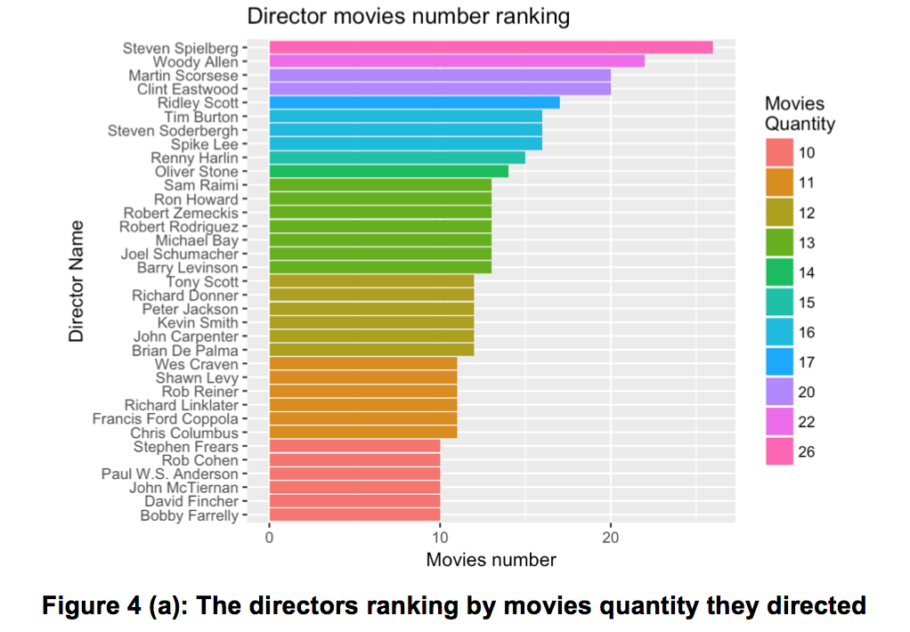
The figure 5(a) above illustrates that the most prolific director is Steven Spielberg☺️ who have directed 26 movies, the other prolific directors included Woody Allen, Martin Scorsese and Clint Eastwood who all directed over 20 movies.
From these 35 directors, a boxplot of them and the IMDB score of their movies were generated, and ranked in descending order by their medians of IMDB scores in figure 5 (b).
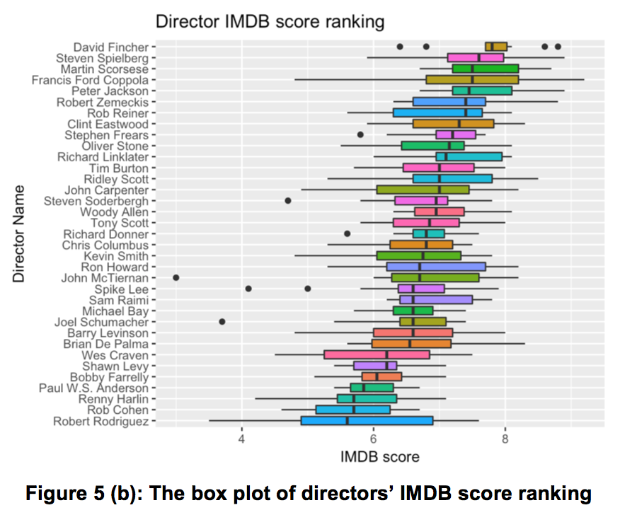
The figure 5(b) above illustrates that the director with highest score is David Fincher, having directed 5 movies with a median IMDB score of 7.8. If we consider both quantity and quality of movies produced, 👍Steven Spielberg is the director that performs well in both respects (1st in quantity, 2nd in score ranking).
# Q5: Director's impact of the imdb scores
q5_data = movies
q5_data %>%
  subset(director_name != "") %>%
  group_by(director_name) %>%
  summarise(director_movies_count = n()) %>%
  filter(director_movies_count >= 10) %>%
  ggplot(aes(x = reorder(director_name, director_movies_count), y = director_movies_count)) +
  geom_bar(stat = "identity", aes(fill = as.factor(director_movies_count))) +
  coord_flip() +
  guides(fill=guide_legend(title="Movies\nQuantity")) +
  labs(x = "Director Name", y = "Movies number", title = "Director movies number ranking")

topDirectors = q5_data %>%
  subset(director_name != "") %>%
  group_by(director_name) %>%
  summarise(director_movies_count = n()) %>%
  filter(director_movies_count >= 10)
directorList = lapply(topDirectors[1], as.factor)

q5_data[q5_data$director_name %in% directorList$director_name, ] %>%
  ggplot(aes(reorder(director_name, imdb_score, median, order = TRUE), y = imdb_score, fill = director_name)) +
  geom_boxplot() +
  guides(fill=FALSE) +
  coord_flip() +
  labs(x = "Director Name", y = "IMDB score", title = "Director IMDB score ranking")
Conclusion
Through visualization and analytics of IMDB 5000 dataset, we focus on 5 issues related to the IMDB scores. During exploration, we emphasize the factors including years (1916 to 2016), 21 types of genres, 66 countries (especially top 20 countries), gross, budget and 35 prolific directors across 5043 movies. After that, some perspectives were made based on data analytics, which were meaningful to summarize and predict the overall movie market tendency. At the same time, the inferences were also beneficial for movie workers to grab audience’s preference effectively.